Making a Better Map Part 2: ggplot and Tigris
Continuing Where we Left Off
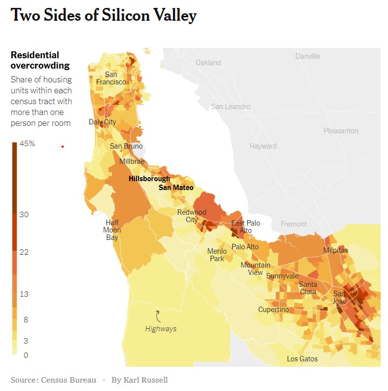
In Part One of this series we worked on getting data using the TidyCensus package to recreate the map below from a recent New York Times Story. Now we’re going to actually do the mapping bit.
It Floats…kind of
So this should be pretty straightforward: we’ve got a dataframe with shapefiles called bay_area_housing. It’s got one column with a shapefile of each census tract in the bay area and another with a ratio of dwellings where more than one person resides per room. Using the geom_sf() function we can make a basic map with just a couple lines of code.
ggplot(data = bay_area_housing) +
geom_sf(color = NA, aes(geometry = geometry, fill = ratio_over_1)) 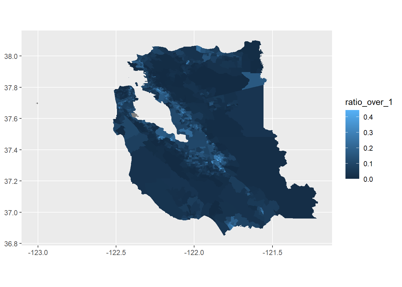
It’s not pretty. At all. And it’s nothing like the map we are trying to replicate. In no particular order, if we want to recreate the map from the NYT, we’re going to need:
1) Roads
2) The landmass outside of our chosen area
3) City Names
4) A better color palette
5) Water. And that water should be blue!
So how do we get all of that?
Enter Tigris
By an almost obscene stroke of luck (and by luck I mean the hard work of the authors), the Tigris library can help us get almost all of these. Seriously, getting all of the data we need for roads, landmass and water is just this simple:
library(tigris)

my_state = 'CA'
my_county = c('San Francisco','San Mateo','Santa Cruz','Santa Clara','Alameda','Contra Costa','Los Angeles')

roads_data = primary_secondary_roads(my_state) %>%
  filter(RTTYP %in% c('U','S','I')) #this will limit the roads to just highways.
landmass_data = counties(cb = TRUE, state = my_state)
water_data = area_water(my_state,my_county)
Let’s see what we can muster now with these supporting layers. Note that I’m moving my data arguments into each individual geom_sf() call since we’re pulling from more than one data frame. Also since these layers will stack on top of eachother, the order that we feed them into ggplot is very important.
my_map = ggplot() +
  theme_void()  + #whiteout
  geom_sf(data = landmass_data, fill = '#e6e6e6', color = NA,aes(geometry = geometry)) + #grey landmass
  geom_sf(data = bay_area_housing, color = NA, aes(geometry = geometry, fill = ratio_over_1)) + #our census map
  geom_sf(data = water_data, fill = '#cce6ff',color = NA, aes(geometry = geometry)) + #add water
  theme(panel.background = element_rect(fill = '#cce6ff', color = NA)) + #blue background to mesh with water
  geom_sf(data = roads_data, color = 'white', aes(geometry = geometry)) + #add roads
  NULL

my_map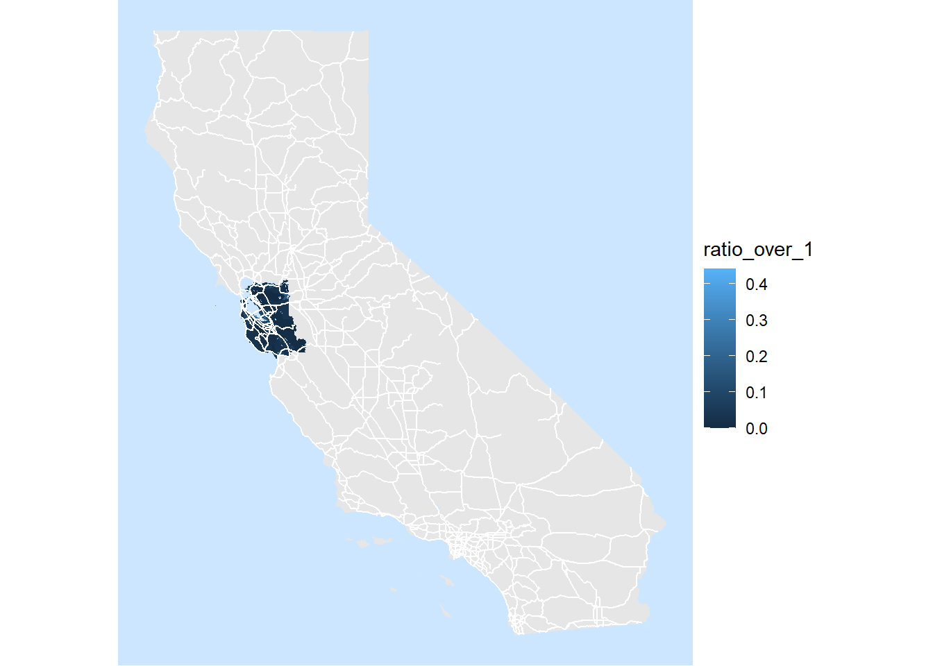
Crap. We’ve got what’s probably a pretty decent map, but it’s for the whole state. This kind of makes sense actually, since some of our calls to Tigris only specify a state and not a county, and ggplot doesn’t know that we only care to frame the parts of the data that are included in our bay_area_housing layer. Luckily there is a way around this. Using the coord_sf() function we can set x and y limits based on our original dataframe. This is kind of tricky since shapefiles don’t behave the way a lot of other R objects do but we can extract them like so using the st_bbox() function contained in the sf library.
limits = st_bbox(bay_area_housing$geometry)
limits
## xmin ymin xmax ymax
## -123.01392 36.85065 -121.20823 38.09988Now lets try again with our new limited frame.
my_map = my_map +
  coord_sf(xlim = c(as.numeric(limits$xmin),as.numeric(limits$xmax)),
           ylim = c(as.numeric(limits$ymin),as.numeric(limits$ymax)))

my_map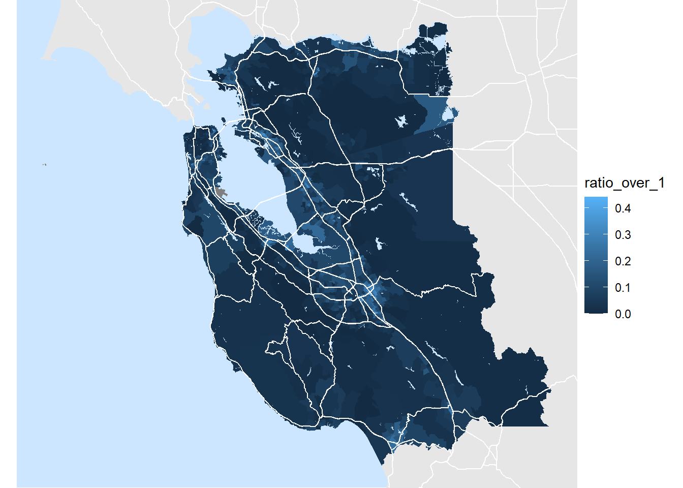
Last Touches
Okay! This is starting to look more professional. We definitely need to get a color scheme that’s a bit more expressive and get our legend a bit more legible. There’s lots of palettes in the viridis library that can make your maps much more legible and accessible but in the spirit of recreating the original map, I’m going to hand pick a gradient to match the levels in the original, while also getting my legend cleaned up.
my_map = my_map +
  labs(fill = 'Share of housing\nunits with more\nthan one person\nper room') + #label legend
  theme(legend.justification = c(0,0), legend.position = c(0.02,0.04)) + # move legend to bottom left
  scale_fill_gradient(low = '#ffff99', high = '#b10026', na.value = '#ffffcc' )  # custom fill palette

my_map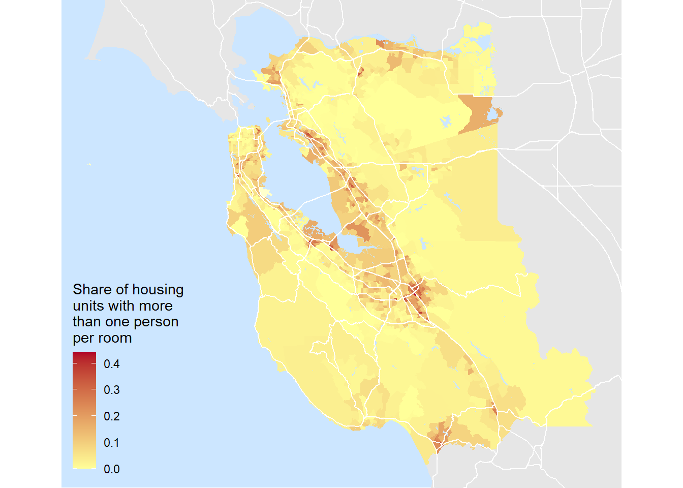
Very nice. All that’s left to do is add our cities and we’ll be all set. I found that one area where Tigris isn’t great is getting simple points for the locations of cities (it really just deals with polygons), but there is a maps package that has built in data for US cities. Lets bring in that data and add in the last layer of our map. In order to keep things from getting too crowded we’ll add a cutoff for cities that are under a certain size.
library(maps)
cities_data = us.cities %>%
  filter(country.etc %in% my_state & pop > 75000)  %>%
  mutate(fixed_name = str_replace(name,country.etc,'')) # this will drop the state name from the name column

my_map +
geom_text(color = 'black',data = cities_data ,check_overlap = TRUE ,aes(x = long, y = lat, label = fixed_name)) 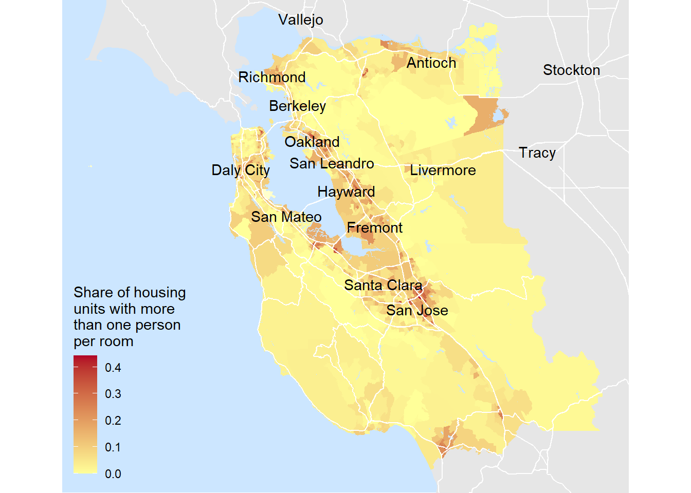
Wow…lets just take minute to recall our journey here. Nicely done!

We Hunger for More Maps
Ok! We’ve recreated the original map. Remember though, one of the goals of this project was to be able to make a tool that we can use to create similar visualizations for ANYWHERE in the US.
Well…if we’re gonna be running the same code several times over, this sounds like a job for a function. This next part is gonna involve a lot of code we’ve already gone over but the basic idea is to make two functions: one to pull the data we need to make the map and one to actually render it. First the data puller: This is going to let us grab our underlying info from the TidyCensus, Tigris and Maps package.
pull_data = function(my_state, my_county){

  acs = load_variables(2018, 'acs5', cache = TRUE)

  concepts = acs %>%
    filter(concept == 'TENURE BY OCCUPANTS PER ROOM')

  concepts_string = concepts %>%
    select(1) %>%
    pull() # this creates a character vector of just the concepts we want


  raw =  get_acs(geography = 'tract', variables = concepts_string, year = 2018, state = my_state,
                 county = my_county,geometry = TRUE, cache = TRUE)

  fixed_data = concepts %>%
    select(name, label) %>%
    right_join(raw, by = c('name' = 'variable')) %>%
    select(2,3,5,7) %>%
    spread(key = label, value = estimate, -4)

  names(fixed_data) = make.names(names(fixed_data))

  fill_data = fixed_data %>%
    mutate(
      total_under_1 = Estimate..Total..Owner.occupied..0.50.or.less.occupants.per.room + Estimate..Total..Owner.occupied..0.51.to.1.00.occupants.per.room + Estimate..Total..Renter.occupied..0.50.or.less.occupants.per.room + Estimate..Total..Renter.occupied..0.51.to.1.00.occupants.per.room,
      total_over_1 = Estimate..Total..Owner.occupied..1.01.to.1.50.occupants.per.room + Estimate..Total..Owner.occupied..1.51.to.2.00.occupants.per.room + Estimate..Total..Owner.occupied..2.01.or.more.occupants.per.room + Estimate..Total..Renter.occupied..1.01.to.1.50.occupants.per.room + Estimate..Total..Renter.occupied..1.51.to.2.00.occupants.per.room + Estimate..Total..Renter.occupied..2.01.or.more.occupants.per.room
    ) %>%
    select(GEOID,geometry ,total_under_1, total_over_1, Estimate..Total) %>%
    mutate(ratio_over_1 = total_over_1/ Estimate..Total)

  roads_data = primary_secondary_roads(my_state) %>%
    filter(RTTYP %in% c('U','S','I'))

  counties_data = counties(cb = TRUE)
  water_data = area_water(my_state,my_county)

  cities_data = us.cities %>%
    filter(country.etc %in% my_state)  %>%
    mutate(fixed_name = str_replace(name,country.etc,'')) # this will drop the state name from the name column

  return(list(fill = fill_data, roads = roads_data, counties = counties_data, water =  water_data, cities = cities_data))
}
Second is the actual mapper. I’ve got two extra parameters in here to make this more flexible for various geographies. One allows you to specify a population cutoff for which cities will be included on the map. Another lets you specify which corner of the map to stick the legend.
mapper = function(input_data, city_size_floor = 100000000, legend_position = 'bottom left'){ #accepts list object from pull_data function
  map_frame = input_data$fill
  limits = st_bbox(map_frame$geometry)
  roads = input_data$roads
  county = input_data$counties
  water = input_data$water
  cities = input_data$cities %>%
    filter(pop > city_size_floor & long > as.numeric(limits$xmin) & long < as.numeric(limits$xmax) &
             lat>(as.numeric(limits$ymin) & lat < as.numeric(limits$ymax)))

  legend_placer = function(position = 'bottom left'){
    if(position == 'bottom left'){
      ret = (list(c(0,0),c(0.02,0.04)))
    }else if(position == 'top left'){
      ret =(list(c(0,1),c(0.02,0.96)))
    }else if (position == 'bottom right'){
      ret=(list(c(1,0),c(0.98,0.04)))
    }else if(position == 'top right'){
      ret=(list(c(1,1),c(0.98,0.96)))
    }else(stop('invalid input: must supply one of: bottom left, bottom right, top left, top right'))
    return(theme(legend.justification = ret[[1]], legend.position = ret[[2]]))
  }

  ggplot() +
    theme_void()  + #whiteout
    legend_placer(legend_position) +
    labs(fill = 'Share of housing\nunits with more\nthan one person\nper room')+ #label legend
    geom_sf(data = county, alpha = 1, fill = '#e6e6e6', color = NA,aes(geometry = geometry)) + #grey landmass
    geom_sf(data = map_frame, alpha = 1,color = NA, aes(geometry = geometry, fill = ratio_over_1)) + #our census map
    scale_fill_gradient(low = '#ffff99', high = '#b10026', na.value = '#ffffcc' ) + # custom fill palette
    geom_sf(data = water, fill = '#cce6ff',color = NA, aes(geometry = geometry)) + #add water
    theme(panel.background = element_rect(fill = '#cce6ff', color = NA)) + #blue background to mesh with water
    geom_sf(data = roads, color = 'white', aes(geometry = geometry)) + #add roads
    geom_text(color = 'black',data = cities,check_overlap = TRUE ,aes(x = long, y = lat, label = fixed_name)) + #add city names
    coord_sf(xlim = c(as.numeric(limits$xmin),as.numeric(limits$xmax)), ylim = c(as.numeric(limits$ymin),as.numeric(limits$ymax))) + #set framing(very important)
    NULL
}
So lets give it a whirl: let’s start with New York City:
nyc = pull_data('NY',c('Bronx','New York','Queens','Kings'))
mapper(nyc, legend_position = 'top left')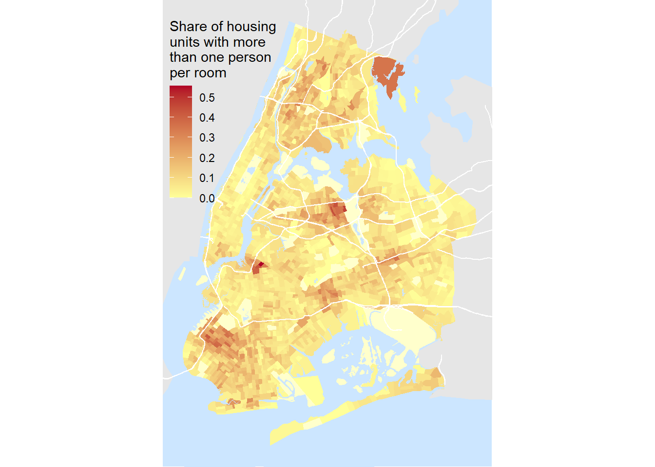
How about my hometown?
atx = pull_data('TX',c('Travis','Williamson','Hays','Caldwell','Bastrop'))
mapper(atx, 40000, legend_position = 'top left')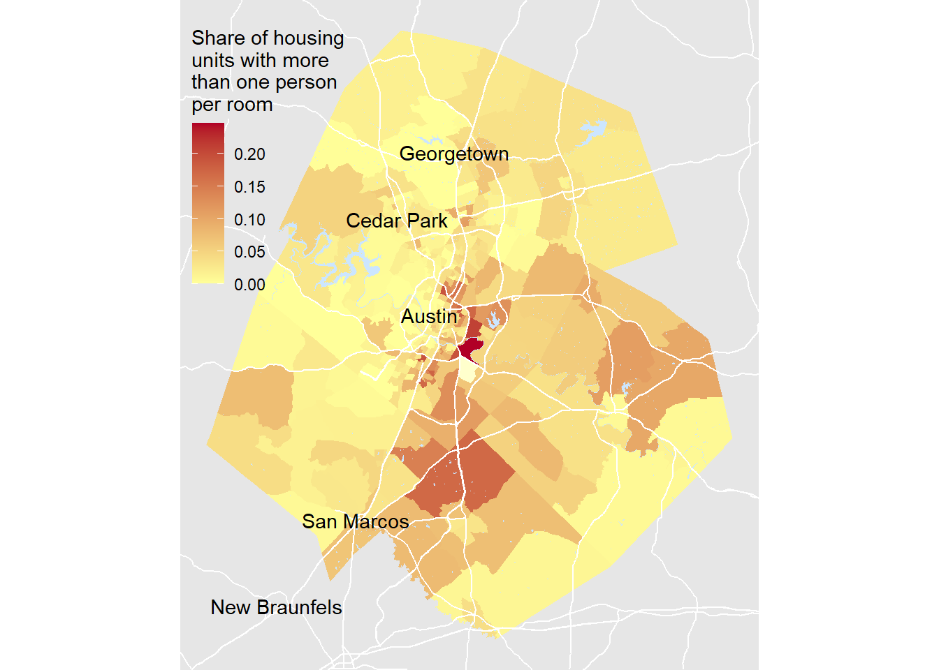
I think we’ve done it. If you want to see maps for your own city or region, feel free to copy my functions and run them locally. If you find a way to improve on them let me know!
